Statistics

What statistics covers

Half of Paper 3 of 9MA0, sat in the same two hours as Mechanics. Data summarised carefully, chance made calculable, two named distributions, and the machinery for deciding whether an effect is real. The Edexcel large data set is examinable here, and a calculator does most of the arithmetic, so the marks sit in the setting up and the conclusions.

The main ideas

• Populations and samples, the five sampling methods with an advantage and a limitation each, and the shape of the large data set.
• Mean, median, quartiles and percentiles by interpolation, variance and standard deviation from the two sums, and undoing coding.
• Histograms with frequency density, cumulative frequency, box plots, skewness, and the quartile fence rule for outliers.
• Scatter diagrams, the product moment correlation coefficient, regression with its interpretation in context, log transformations, and the limits of prediction.
• Venn diagrams and the addition rule, mutual exclusivity against independence, then conditional probability, trees without replacement and two-way tables.
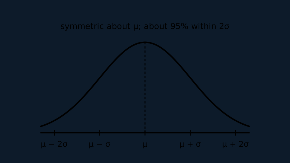
• The binomial distribution with its four conditions, and the normal distribution with standardising, the inverse normal and the approximation to the binomial.
• Hypothesis testing: hypotheses stated in the parameter, one and two tails, critical regions and actual significance levels, extended to a correlation coefficient and to a normal mean.

The results it turns on

σ² = Σx²/n − (Σx/n)²

variance worked straight from the two given sums

area is frequency, so frequency density = frequency ÷ class width

reading and drawing a histogram

fences at Q₁ − 1.5 × IQR and Q₃ + 1.5 × IQR

the outlier rule, learned as a sentence

P(A ∪ B) = P(A) + P(B) − P(A ∩ B), and P(A|B) = P(A ∩ B)/P(B)

the addition rule and conditional probability

X ~ B(n, p), and Z = (X − μ)/σ

naming a binomial model, and standardising a normal variable

the mean of n readings is N(μ, σ²/n)

the distribution a test on a normal mean standardises with

Where it usually goes wrong

• Mutually exclusive and independent are different properties, and a pair of events with positive probabilities can rarely be both. Independence is settled by comparing the overlap with the product, shown on the page.
• For a two-tailed test the significance level is halved before any comparison, and this is one of the commonest ways to lose a mark in the section.
• A test uses the probability of a result at least as extreme, which is a tail probability. Testing the probability of the observed value alone answers a different question.
• The inverse normal takes the area to the left, so the top 15 per cent becomes 0.85 before anything is typed in.

Where to start

Sampling first, then location and spread, then representation, since the three make one block on summarising data. Correlation and regression next. Probability and conditional probability form a second block, and the two distributions a third. Leave hypothesis testing until last: both of its lessons call on everything before them.